Page 57 - 4660

Important continuous distributions

f(x)

0.4

0.3
Φ(a)
0.2

0.1
a
x
−4 −3 −2 −1 0 1 2 3 4
Φ(x)
1
Φ(a)

0.5

a
x
−4 −3 −2 −1 1 2 3 4

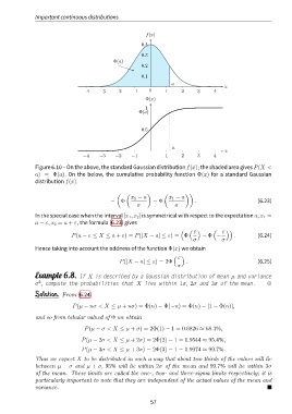
Figure 6.10 – On the above, the standard Gaussian distribution f(x); the shaded area gives P(X <
a) = Φ(a). On the below, the cumulative probability function Φ(x) for a standard Gaussian
distribution f(x).

( ( ) ( ))
x 2 − a x 1 − a
= Φ − Φ . (6.23)
σ σ
In the special case when the interval [x 1 , x 2 ] is symmetrical with respect to the expectation a, x 1 =
a − ε, x 2 = a + ε, the formula (6.23) gives
ε ε
( ( ) ( ))
P(a − ε ≤ X ≤ a + ε) = P(|X − a| ≤ ε) = Φ − Φ − . (6.24)
σ σ
Hence taking into account the oddness of the function Φ(x) we obtain

ε
( )
P(|X − a| ≤ ε) = 2Φ . (6.25)
σ
Example 6.8. If X is described by a Gaussian distribution of mean µ and variance
2
σ , compute the probabilities that X lies within 1σ, 2σ and 3σ of the mean. ,
Solution. From (6.24)

P(µ − nσ < X ≤ µ + nσ) = Φ(n) − Φ(−n) = Φ(n) − [1 − Φ(n)],

and so from tabular valued of Φ we obtain

P(µ − σ < X ≤ µ + σ) = 2Φ(1) − 1 = 0.6826 ≈ 68.3%,

P(µ − 2σ < X ≤ µ + 2σ) = 2Φ(2) − 1 = 0.9544 ≈ 95.4%,
P(µ − 3σ < X ≤ µ + 3σ) = 2Φ(3) − 1 = 0.9974 ≈ 99.7%.

Thus we expect X to be distributed in such a way that about two thirds of the values will lie
between µ − σ and µ + σ, 95% will lie within 2σ of the mean and 99.7% will lie within 3σ
of the mean. These limits are called the one-, two- and three-sigma limits respectively; it is
particularly important to note that they are independent of the actual values of the mean and
variance.

57