Page 56 - 4660

Continuous random variables

1. f(x) > 0 for all x ∈ R.

2
(x−a)
1
2. The function f(x) has the maximum at x = a, equals √ . Really f (x) = − x−a − 2σ 2 .
′
√ e
σ 2π σ 3 2π
Therefore f (x) = 0 if x = a, hence f (x) > 0 for x < a, and f (x) < 0 for x > a. This means
′
′
′
1
that x = a is the point of maximum and f max = f(a) = √ .
σ 2π
3. Calculating the second derivative of f(x) we can verify that the points x = a ± σ are points
of inflexion.
4. The graph of the function is symmetric with respect to the vertical straight line x = a.
5. lim f(x) = 0, that is OX axes is a horizontal asymptote of the function f(x).
x→∞
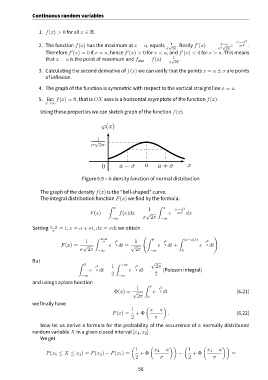
Using these properties we can sketch graph of the function f(x).

ϕ(x)

1
√
σ 2π

0 a − σ a a + σ x

Figure 6.9 – A density function of normal distribution

The graph of the density f(x) is the “bell-shaped” curve.
The integral distribution function F(x) we find by the formula:

∫ ∫
x 1 x (x−a) 2
F(x) = f(x)dx = √ e − 2σ 2 dx
σ 2π
−∞ −∞
Setting x−a = t; x = a + σt, dx = σdt we obtain
σ
( )
∫ x−a ∫ 0 ∫ (x−a)/σ
1 σ t 2 1 t 2 t 2
F(x) = √ e − 2 dt = √ e − 2 dt + e − 2 dt .
σ 2π −∞ 2π −∞ 0
But
∫ ∫ √
0 +∞
t 2 1 t 2 2π
e − 2 dt = e − 2 dt = (Poisson integral)
2 2
−∞ −∞
and using Laplace function
∫ x
1 t 2
Φ(x) = √ e − 2 dt (6.21)
2π 0
we finally have
( )
1 x − a
F(x) = + Φ . (6.22)
2 σ
Now let us derive a formula for the probability of the occurrence of a normally distributed
random variable X in a given closed interval [x 1 , x 2 ].
We get

( ( )) ( ( ))
1 x 2 − a 1 x 1 − a
P(x 1 ≤ X ≤ x 2 ) = F(x 2 ) − F(x 1 ) = + Φ − + Φ =
2 σ 2 σ

56