Page 54 - 4660

Continuous random variables

y

k

0 x

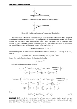
Figure 6.6 – A density function of exponential distribution

y

1

0 x

Figure 6.7 – An integral function of exponential distribution

The exponential distribution occurs naturally if we consider the distribution of the length of
intervals between successive events in a Poisson process or, equivalently, the distribution of the
interval (i.e. the waiting time) before the first event. If the average number of events per unit
interval is k then on average there are kx events in interval x, so that from the Poisson distribution
the probability that there will be no events in this interval is given by

P(no events in interval x) = e −kx .

The probability that an event occurs in the next infinitestimal interval [x, x + dx] is given by kdx,
so that
P(the first event occurs in interval [x, x + dx]) = e −kx kdx.
Hence the required probability density function is given by

f(x) = ke −kx .

Now we find the mean and the variance
∫ ∫ b
+∞ integrating
E(X) = xke −kx dx = lim xke −kx dx = =
by parts
0 b→+∞ 0
( )
1 b 1 1
= lim −xe −kx − e −kx = 0 − (0 − 1) = .
b→+∞ k 0 k k

∫ ∫
+∞ +∞ 1 integrating by
2
2 −kx
2 −kx
Var(X) = x e dx − M (X) = k x e dx − 2 = parts twice =
−∞ 0 k
( 2 ( ))
x 2 x 1 b 1
= k lim − e −kx + − e −kx − e −kx − =
k k k k 2 0 k 2
x→+∞
( ( ))
2 1 1 2 1 1
= k 0 − 0 + 0 − (0 − 1) − = − = .
k k 2 k 2 k 2 k 2 k 2
Thus
1 1 1
E(X) = , Var(X) = , σ(X) = . (6.17)
k k 2 k
Example 6.7. Let T be a time period of operating a radio bulb, which has an
exponential distribution. Find the probability of operating a radio bulb not less
than 800 hours if an average time period is 400 hours. ,

54