Page 59 - 4660

Important continuous distributions

Now using Φ(−z) = 1 − Φ(z) gives

( )
µ − 140
Φ = 1 − 0.030 = 0.970.
σ

We find that
µ − 140
= 1.88. (6.27)
σ
Solving the simultaneous equations (6.26) and (6.27) gives µ = 173.5, σ = 17.8.

From the above examples, we see that the kurtosis of the Gaussian distribution is given by
γ 4 = ν 4 2 = 2σ 4 = 3. It is therefore common practice to define the excess kurtosis of a
ν 2 σ 4
distribution as γ 4 − 3. A positive value of the excess kurtosis implies a relatively narrower peak
and wider wings than the Gaussian distribution with the same mean and variance. A negative
excess kurtosis implies a wider peak and shorter wings.

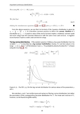
The log-normal distribution. If the random variable X follows a Gaussian distribution then the
X
variable Y = e is described by a log-normal distribution. Clearly, if X can take values in the
range −∞ to ∞, then Y will lie between 0 and ∞. The probability density function for Y is found
using the result (6.14). It is

[ 2 ]
dx 1 1 (ln y − µ)

g(y) = f(x(y)) = √ exp − .
dy σ 2π y 2σ 2

g(y)

1 µ = 0, σ = 0.5
µ = 0, σ = 1
µ = 0, σ = 1.5
0.8

0.6

0.4

0.2

0 y
0 1 2 3 4

Figure 6.11 – The PDF g(y) for the log-normal distribution for various values of the parameters µ
and σ.

2
We note that µ and σ are not the mean and variance of the log-normal distribution, but rather
the parameters of the corresponding Gaussian distribution for X. The mean and variance of Y,
however, can be found straightforwardly

1
2
E(Y ) = exp(µ + σ ),
2

2
2
Var(Y ) = exp(2µ + σ )[exp(σ ) − 1].
59