Page 61 - 4660

Important continuous distributions

f(x)

1 x 0 = 0, Γ = 1
x 0 = 2, Γ = 1
x 0 = 0, Γ = 3
0.8

0.6

0.4

0.2

x
−4 −2 0 2 4

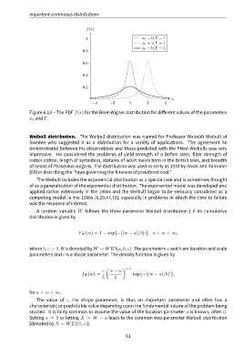
Figure 6.13 – The PDF f(x) for the Breit-Wigner distribution for different values of the parameters
x 0 and Γ.

Weibull distribution. The Weibull distribution was named for Professor Waloddi Weibull of
Sweden who suggested it as a distribution for a variety of applications. The agreement he
demonstrated between his observations and those predicted with the fitted Weibulls was very
impressive. He considered the problems of yield strength of a Bofors steel, fiber strength of
Indian cotton, length of syrtoideas, statures of adult males born in the British Isles, and breadth
of beans of Phaseolus vulgaris. The distribution was used as early as 1933 by Rosin and Rammler
[69] in describing the ‘‘laws governing the fineness of powdered coal.’’
The Weibull includes the exponential distribution as a special case and is sometimes thought
of as a generalization of the exponential distribution. The exponential model was developed and
applied rather extensively in the 1950s and the Weibull began to be seriously considered as a
competing model in the 1960s [6,29,47,73], especially in problems in which the time to failure
was the response of interest.

A random variable W follows the three-parameter Weibull distribution [ if its cumulative
distribution is given by

F W (w) = 1 − exp{−[(w − a)/b]c}, a < w < ∞,

where b, c > 0. It is denoted by W ∼ WE3(a, b, c). The parameters a and b are location and scale
parameters and c is a shape parameter. The density function is given by

( ) c−1
c w − a
c
f W (w) = exp{−[(w − a)/b] },
b b

for a < w < ∞.

The value of c, the shape parameter, is thus an important parameter and often has a
characteristic or predictable value depending upon the fundamental nature of the problem being
studied. It is fairly common to assume the value of the location parameter a is known, often 0.
Setting a = 0 or letting X = W − a leads to the common two-parameter Weibull distribution
[denoted by X ∼ WE2(b, c)].

61