Page 58 - 4660

Continuous random variables

There are many other ways in which the Gaussian distribution may be used. We now illustrate
some of the uses in more complicated examples.

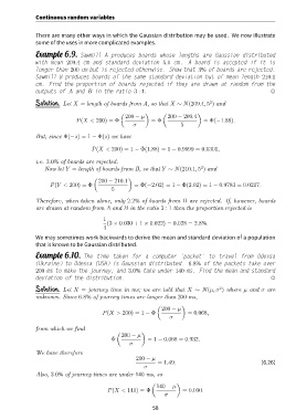
Example 6.9. Sawmill A produces boards whose lengths are Gaussian distributed
with mean 209.4 cm and standard deviation 5.0 cm. A board is accepted if it is
longer than 200 cm but is rejected otherwise. Show that 3% of boards are rejected.
Sawmill B produces boards of the same standard deviation but of mean length 210.1
cm. Find the proportion of boards rejected if they are drawn at random from the
outputs of A and B in the ratio 3 : 1. ,

2
Solution. Let X = length of boards from A, so that X ∼ N(209.4, 5 ) and
( ) ( )
200 − µ 200 − 209.4
P(X < 200) = Φ = Φ = Φ(−1.88).
σ 5

But, since Φ(−z) = 1 − Φ(z) we have

P(X < 200) = 1 − Φ(1.88) = 1 − 0.9699 = 0.0301,

i.e. 3.0% of boards are rejected.
2
Now let Y = length of boards from B, so that Y ∼ N(210.1, 5 ) and
( )
200 − 210.1
P(Y < 200) = Φ = Φ(−2.02) = 1 − Φ(2.02) = 1 − 0.9783 = 0.0217.
5

Therefore, when taken alone, only 2.2% of boards from B are rejected. If, however, boards
are drawn at random from A and B in the ratio 3 : 1 then the proportion rejected is
1
(3 × 0.030 + 1 × 0.022) = 0.028 = 2.8%.
4

We may sometimes work backwards to derive the mean and standard deviation of a population
that is known to be Gaussian distributed.

Example 6.10. The time taken for a computer ’packet’ to travel from Odessa
(Ukraine) to Odessa (USA) is Gaussian distributed. 6.8% of the packets take over
200 ms to make the journey, and 3.0% take under 140 ms. Find the mean and standard
deviation of the distribution. ,

2
Solution. Let X = journey time in ms; we are told that X ∼ N(µ, σ ) where µ and σ are
unknown. Since 6.8% of journey times are longer than 200 ms,
( )
200 − µ
P(X > 200) = 1 − Φ = 0.068,
σ

from which we find
( )
200 − µ
Φ = 1 − 0.068 = 0.932.
σ
We have therefore
200 − µ
= 1.49. (6.26)
σ
Also, 3.0% of journey times are under 140 ms, so

( )
140 − µ
P(X < 140) = Φ = 0.030.
σ

58