Page 60 - 4660

Continuous random variables

The chi-squared distribution. Above we showed that if X is Gaussian distributed with mean µ
2
2
2
2
and variance σ , such that X ∼ N(µ, σ ), then the random variable Y = (x−µ) /σ is distributed
1 1
as the gamma distribution Y ∼ γ( , ). Let us now consider n independent Gaussian random
2 2
2
variables X i ∼ N(µ i , σ ), i = 1, 2, . . . , n, and define the new variable
i
n 2
∑ (X i − µ i )
2
χ = 2 . (6.28)
n
i=1 σ i
2
1 1
2
It can be proved that χ must be distributed as the gamma variate χ ∼ γ( , n), which from
n
n
2 2
(6.18) has the PDF
( ) n/2−1 ( ) ( )
1/2 1 1 1 1
2 n/2−1
2
f(χ ) = ( ) χ 2 exp − χ 2 n = (χ ) exp − χ 2 n . (6.29)
n
n
n
1
Γ 1 n 2 2 2 n/2 Γ( n) 2
2 2
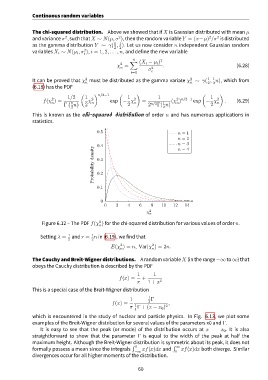
This is known as the chi-squared distribution of order n and has numerous applications in
statistics.
0.5 n = 1
n = 2
n = 3
0.4
density 0.3 n = 4
Probability 0.2
0.1
0
0 2 4 6 8 10 12 14
χ 2
n
2
Figure 6.12 – The PDF f(χ ) for the chi-squared distribution for various values of order n.
n
1
Setting λ = 1 and r = n in (6.19), we find that
2 2
2
2
E(χ ) = n, Var(χ ) = 2n.
n
n
The Cauchy and Breit-Wigner distributions. A random variable X (in the range −∞ to ∞) that
obeys the Cauchy distribution is described by the PDF
1 1
f(x) = +
π 1 + x 2

This is a special case of the Breit-Wigner distribution
1 1 Γ
f(x) = 2 ,
1
π Γ + (x − x 0 ) 2
4
which is encountered in the study of nuclear and particle physics. In Fig. 6.13, we plot some
examples of the Breit-Wigner distribution for several values of the parameters x0 and Γ.
It is easy to see that the peak (or mode) of the distribution occurs at x = x 0 . It is also
straightforward to show that the parameter Γ is equal to the width of the peak at half the
maximum height. Although the Breit-Wigner distribution is symmetric about its peak, it does not
∫ 0 ∫
formally possess a mean since the integrals xf(x)dx and ∞ xf(x)dx both diverge. Similar
−∞ 0
divergences occur for all higher moments of the distribution.

60