Page 53 - 4660

Important continuous distributions

∫ ∫ ∫
a b dt x b − a
= 0dt + + odt = = 1.
b − a b − a
−∞ a b
Therefore

0, if x < a,

F(x) = x−a , if a ≤ x ≤ b,
b−a


1, if b < x.
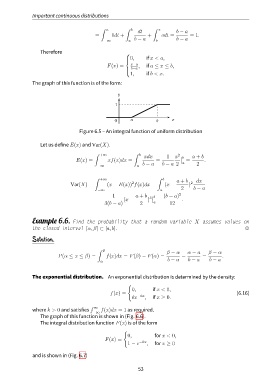
The graph of this function is of the form:

y
1

0 a b x

Figure 6.5 – An integral function of uniform distribution

Let us define E(x) and Var(X).
∫ ∫ b
+∞ xdx 1 x 2 b a + b
E(x) = xf(x)dx = = = .
b − a b − a 2 a 2
−∞ a

∫ ∫ b
+∞ a + b dx
2
Var(X) = (x − E(x)) f(x)dx = (x − ) 2 =
2 b − a
−∞ a
1 a + b b (b − a) 2
= (x − ) 3 = .
3(b − a) 2 a 12

Example 6.6. Find the probability that a random variable X assumes values on
the closed interval [α, β] ⊂ [a, b]. ,
Solution.

∫
β β − α α − a β − α
P(α ≤ x ≤ β) = f(x)dx = F(β) − F(α) = − = .
α b − a b − a b − a

The exponential distribution. An exponential distribution is determined by the density:

{
0, if x < 0,
f(x) = (6.16)
ke −kx , if x ≥ 0.

∫ ∞
where k > 0 and satisfies f(x)dx = 1 as required.
−∞
The graph of this function is shown in (Fig. 6.6).
The integral distribution function F(x) is of the form

{
0, for x < 0,
F(x) =
1 − e −kx , for x ≥ 0

and is shown in (Fig. 6.7)

53