Page 50 - 4660

Continuous random variables

′
Solution. First of all we find the density distribution function f(x) = F (x).

0, if x ≤ 0,

f(x) = 1 , if 0 < x ≤ 2,
2


0, if x > 2.
∫ ∫ 0 ∫ 2 ∫ ∫ 2
+∞ 1 +∞ 1 x 2 2
E(X) = xf(x)dx = x · 0dx + x · dx + x · 0dx = xdx = 0 = 1.
−∞ −∞ 0 2 2 2 0 4
∫ ∫ 2
+∞ 1 (x − 1) 3 2 1
2
2
Var(X) = (x − 1) f(x)dx = (x − 1) · dx = 0 = .
−∞ 0 2 6 3
√ 1
σ = Var(X) = √ .
3

Function of continuous random variable

If X is a continuous RV, then so too is the new random variable Y = Y (X). The probability that Y
lies in the range y to y + dy is given by
∫
g(y)dy = f(x)dx, (6.13)
dS
where dS corresponds to all values of x for which Y lies in the range y to y + dy. Once again the
simplest case occurs when Y (X) possesses a single-valued inverse X(Y ). In this case, we may
write

∫ ∫ dx
x(y+dy) x(y)+| |dy
dy
′
′
′
′
f(x )dx = f(x )dx ,
g(y)dy =

x(y) x(y)
from which we obtain

dx
g(y) = f(x(y)) . (6.14)
dy

lighthouse
θ
beam
L

y
0 coastline

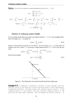
Figure 6.3 – The illumination of a coastline by the beam from a lighthouse

Example 6.4. A lighthouse is situated at a distance L from a straight coastline,
opposite a point O, and sends out a narrow continuous beam of light simultaneously
in opposite directions. The beam rotates with constant angular velocity. If the
random variable Y is the distance along the coastline, measured from O, of the
spot that the light beam illuminates, find its probability density function. ,

50