Page 48 - 4660

Continuous random variables

2.
∫
x 2
P(x 1 < X < x 2 ) = f(x)dx. (6.5)
x 1
Since F (x) = f(x) then F(x) is an antiderivative of a function f(x). Using the Newton-
′
Leibnitz formula we have
∫
x 2
P(x 1 < X < x 2 ) = F(x 2 ) − F(x 1 ) = f(x)dx.
x 1

f(x)

x
0 a x 2 x 1 b

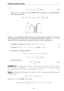
Figure 6.2 – The probability density function for a continuous random variable X that can take
values only between the limits a and b. The shaded area under the curve gives P(x 1 < X ≤ b),
whereas the total area under the curve, between the limits a and b, is equal to unity.

∫ +∞
Corollary 6.3. Really f(x)dx = P(−∞ < X < +∞) = 1. 2
−∞
Corollary 6.4. P(a < X < b) = f(c) · (b − a), where c ∈ [a, b]. 2

3. Let a density f(x) be given. Find F(x).

P(−∞ < X < x) = F(x) − F(−∞) = F(x).

∫
x
P(−∞ < X < x) = f(x)dx.
−∞
From this it follows
x
∫
F(x) = f(x)dx. (6.6)
−∞

Example 6.2. A random variable X has a PDF f(x) given by Ae −x in the interval
0 < x < ∞ and zero elsewhere. Find the value of the constant A and hence compute
the probability that X lies in the interval 1 < X ≤ 2. ,

Solution. We require the integral of f(x) between 0 and ∞ to equal unity. Evaluating this
integral, we find
∫
∞
−x −x ∞
Ae dx − [−Ae ]| 0 = A,
0
and hence A = 1. From (6.5), we then obtain

∫ ∫
2 2
−1
−x
P(1 < X ≤ 2) = f(x)dx = e dx = −e −2 − (−e ) = 0.23.
1 1

48