Page 43 - 4660

Important discrete distributions

f(x)
λ = 1 f(x) λ = 2

0.30 0.30

0.20 0.20

0.10 0.10

0.00 x 0.00 x
0 1 2 3 4 5 0 1 2 3 4 5 6 7

f(x) λ = 5
0.30

0.20

0.10

0.00 x
0 1 2 3 4 5 6 7 8 9 10 11
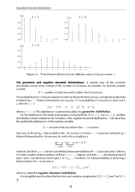
Figure 5.4 – Three Poisson distributions for different values of the parameter λ.

The geometric and negative binomial distributions. A special case of the binomial
distribution occurs when instead of the number of successes we consider the discrete random
variable
X = number of trials required to obtain the first success.
Theprobabilitythatxtrialsarerequiredinordertoobtainthefirstsuccess,issimplytheprobability
of obtaining x − 1 failures followed by one success. If the probability of a success on each trial is
p, then for x > 0
f(x) = P(X = x) = (1 − p) x−1 p = q x−1 p,
where q = 1 − p. This distribution is sometimes called the geometric distribution.
1
For this distribution the mean and variance are found to be E(X) = , Var(X) = q 2 . Another
p p
distribution closely related to the binomial is the negative binomial distribution. This describes
the probability distribution of the random variable

X = number of failures before the r − th success.

One way of obtaining x failures before the r-th success is to have r − 1 successes followed by x
failures followed by the r-th success, for which the probability is

r x
pp · · · p × qq · · · q ×p = p q .
| {z } | {z }
r−1 times x times
However, the first r+x−1 factors constitute just one permutation of r−1 successes and x failures.
The total number of permutations of these r + x − 1 objects, of which r − 1 are identical and of
x
type 1 and x are identical and of type 2, is C r+x−1 . Therefore, the total probability of obtaining x
failures before the r-th success is

x
r x
f(x) = P(X = x) = C r+x−1 p q ,
which is called the negative binomial distribution.
It is straightforward to show that its mean and variance are given by E(X) = rq and Var(X) =
rq p
p 2 .

43