Page 44 - 4660

Discrete random variables

p = 0.2
p = 0.5
P(X = x)
P(X = x)
0.40
0.40

0.20 0.20

0.00 x 0.00 x
0 1 2 3 4 5 0 1 2 3 4 5
P(X = x)
0.80

0.60
p = 0.8

0.40

0.20

0.00 x
0 1 2 3 4 5

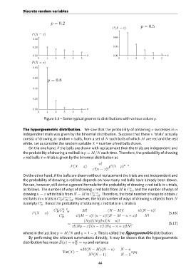
Figure 5.5 – Some typical geometric distributions with various values p.

The hypergeometric distribution. We saw that the probability of obtaining x successes in n
independent trials was given by the binomial distribution. Suppose that these n ’trials’ actually
consist of drawing at random n balls, from a set of N such balls of which M are red and the rest
white. Let us consider the random variable X = number of red balls drawn.
On the one hand, if the balls are drawn with replacement then the trials are independent and
the probability of drawing a red ball is p = M/N each time. Therefore, the probability of drawing
x red balls in n trials is given by the binomial distribution as

n!
x
P(X = x) = p (1 − p) n−x .
x!(n − x)!
On the other hand, if the balls are drawn without replacement the trials are not independent and
the probability of drawing a red ball depends on how many red balls have already been drawn.
We can, however, still derive a general formula for the probability of drawing x red balls in n trials,
x
as follows. The number of ways of drawing x red balls from M is C , and the number of ways of
M
drawing n − x white balls from N − M is C n−x . Therefore, the total number of ways to obtain x
N−M
n−x
x
red balls in n trials is C C N−M . However, the total number of ways of drawing n objects from N
M
n
is simply C . Hence the probability of obtaining x red balls in n trials is
N
x
C C n−x M! (N − M)! n!(N − n)!
P(X = x) = M N−M = = (5.16)
n
C N x!(M − x)! (n − x)!(N − M − n + x)! N!
(Np)!(Nq)!n!(N − n)!
= , (5.17)
x!(Np − x)!(n − x)!(Nq − n + x)!N!
where in the last line p = M/N and q = 1 − p. This is called the hypergeometric distribution.
By performing the relevant summations directly, it may be shown that the hypergeometric
distribution has mean E(x) = n M = np and variance
N
nM(N − M)(N − n) N − n
Var(X) = = npq.
2
N (N − 1) N − 1
44