Page 64 - 4660

Random vectors

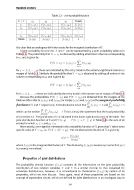
Table 1.3 – Joint probability table

X \ Y y 1 y 2 · · · y n Totals
f(x 1 , y 1 ) f(x 1 , y 2 ) f(x 1 , y n ) f X (x 1 )
x 1 · · ·
f(x 2 , y 1 ) f(x 2 , y 2 ) · · · f(x 2 , y n ) f X (x 2 )
x 2
. . . . . . . . . . . . . . . . . .
f(x m , y 1 ) f(x m , y 2 ) · · · f(x m , y m ) f X (x m )
x m
Totals f Y (y 1 ) f Y (y 2 ) · · · f Y (y n ) 1

It is clear that an analogous definition exists for the marginal distribution of Y.
A joint probability function for X and Y can be represented by a joint probability table as in
Table 1.3. The probability that X = x j is obtained by adding all entries in the row corresponding
to x j and is given by
n
∑
P(X = x j ) = f X (x j ) = f(x j , y k )
k=1
for j = 1, 2, . . . , m these are indicated by the entry totals in the extreme right-hand column or
margin of Table 1.3. Similarly the probability that Y = y k is obtained by adding all entries in the
column corresponding to y k and is given by

m
∑
P(Y = y k ) = f Y (y k ) = f(x j , y k )
j=1

For k = 1, 2, . . . , n these are indicated by the entry totals in the bottom row or margin of Table 1.3.
Because the probabilities P(X = x j ) and P(Y = y k ) are obtained from the margins of the
table we often refer to f X (x j ) and f Y (y k ) (or simply f X (x) and f Y (y)) as themarginal probability
m n
∑ ∑
functions of X and Y respectively. It should also be noted that f X (x j ) = 1 and f Y (y k ) = 1
j=1 k=1
m n
∑ ∑
which can be written f(x j , y k ) = 1 This is simply the statement that the total probability
j=1 k=1
of all entries is 1. The grand total of 1 is indicated in the lower right-hand corner of the table. The
joint distribution function of X and Y F(x, y) = P(X ≤ x, Y ≤ y) in Table 1.3 is the sum of all
entries for which x j ≤ x and y k ≤ y.
Alternatively, one might be interested in the probability function of X given that Y takes some
specific value of Y = y 0 , i.e. P(X = x|Y = y 0 ). This conditional distribution of X is given by

f(x, y 0 )
g(x) = ,
f Y (y 0 )

where f Y (y) is the marginal distribution of Y. The division by f Y (y 0 ) is necessary in order that g(x)
is properly normalized.

Properties of joint distributions

The probability density function f(x, y) contains all the information on the joint probability
distribution of two random variables X and Y. In a similar manner to that presented for
univariate distributions, however, it is conventional to characterize f(x, y) by certain of its
properties, which we now discuss. Once again, most of these properties are based on the
concept of expectation values, which are defined for joint distributions in an analogous way to

64