Page 42 - 4660

Discrete random variables

Example 5.5. The probability of getting exactly 2 heads in 6 tosses of a fair
coin is
2
( ) ( ) 6−2 ( ) 6
1 1 6! 1 15
P(X = 2) = C 2 = = .
6
2 2 2!4! 2 64

f(x)

0.40
n = 5, p = 0.6
f(x) n = 5, p = 0.167
0.30
0.30

0.20
0.20
0.10
0.10

0.00 x 0.00 x
0 1 2 3 4 5 0 1 2 3 4 5
f(x) f(x)
0.40 0.40

n = 10, p = 0.6 n = 10, p = 0.167
0.30 0.30

0.20 0.20

0.10 0.10

0.00 x 0.00 x
0 1 2 3 4 5 6 7 8 9 10 0 1 2 3 4 5 6 7 8 9 10
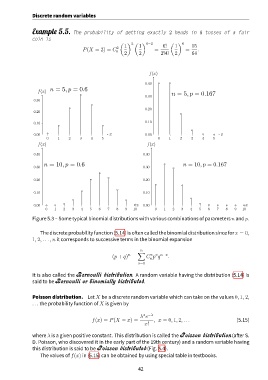
Figure 5.3 – Some typical binomial distributions with various combinations of parameters n and p.

The discrete probability function (5.14) is often called the binomial distribution since for x = 0,
1, 2, . . . , n it corresponds to successive terms in the binomial expansion

n
∑
n
x x n−x
(p + q) = C p q .
n
x=0
It is also called the Bernoulli distribution. A random variable having the distribution (5.14) is
said to be Bernoulli or binomially distributed.

Poisson distribution. Let X be a discrete random variable which can take on the values 0, 1, 2,
. . . the probability function of X is given by

x −λ
λ e
f(x) = P(X = x) = , x = 0, 1, 2, . . . (5.15)
x!
where λ is a given positive constant. This distribution is called the Poisson distribution (after S.
D. Poisson, who discovered it in the early part of the 19th century) and a random variable having
this distribution is said to be Poisson distributed (Fig. 5.4).
The values of f(x) in (5.15) can be obtained by using special table in textbooks.

42