Page 84 - 4811

Solving Systems of Differential Equation Using Laplace Transform
.

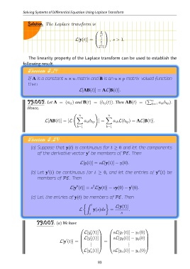
Solution. The Laplace transform is

 
6
s 3
L[y(t)] =  1  , s > 1.
s
1
s−1
. . . .

The linearity property of the Laplace transform can be used to establish the
following result.
Theorem 5.1È

If A is a constant n × n matrix and B is an n × p matrix-valued function
then
L[AB(t)] = AL[B(t)].
. . . . . . .

∑ n
PROOF. Let A = (a ) and B(t) = (b (t)). Then AB(t) = ( k=1 a b ).
ij
ik kp
ij
Hence,
( )
n n
∑ ∑
L[AB(t)] = [L a b ] = a L(b ) = AL[B(t)].
ik kp
ik
kp
k=1 k=1
. . . .
Theorem 5.2È

(a) Suppose that y(t) is continuous for t ≥ 0 and let the components
of the derivative vector y be members of PE. Then
′

L[y(t)] = sL[y(t)] − y(0).

′
′′
(b) Let y (t) be continuous for t ≥ 0, and let the entries of y (t) be
members of PE. Then
2
′′
′
L[y (t)] = s L[y(t)] − sy(0) − y (0).
(c) Let the entries of y(t) be members of PE. Then

t L[y(t)]
{∫ }
L y(s)ds = .
. . . . . . . 0 s

PROOF. (a) We have

   
L[y (t)] sL[y (t)] − y (0)
′
1 1 1
L[y (t)] sL[y (t)] − y (0)
 ′   
′  2   2 2 
L[y (t)] =  . .  =  . . 
 .   . 
′
L[y (t)] sL[y (t)] − y (0)
. . . . n n n
83