Page 109 - 4660

Fisher’s F-test

f(x; d 1 , d 2 )

d 1 = 1, d 2 = 1
2
d 1 = 100, d 2 = 100
d 1 = 5, d 2 = 2
1.5

1

0.5

0 x
0 1 2 3 4

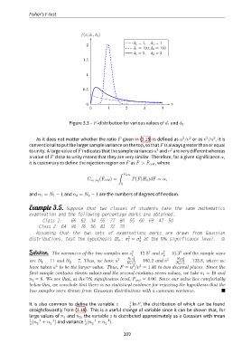
Figure 3.3 – F-distribution for various values of d 1 and d 2 .

2
2
2
2
As it does not matter whether the ratio F given in (3.15) is defined as u /v or as v /u , it is
conventional to put the larger sample variance on the top, so that F is always greater than or equal
2
2
to unity. A large value of F indicates that the sample variances u and v are very different whereas
a value of F close to unity means that they are very similar. Therefore, for a given significance α,
it is customary to define the rejection region on F as F > F crit , where
∫
F crit
(F crit ) = P(F|H 0 )dF = α,
C n 1 ,n 2
1
and n 1 = N 1 − 1 and n 2 = N 2 − 1 are the numbers of degrees of freedom.

Example 3.5. Suppose that two classes of students take the same mathematics
examination and the following percentage marks are obtained:
Class 1: 66 62 34 55 77 80 55 60 69 47 50
Class 2: 64 90 76 56 81 72 70
Assuming that the two sets of examinations marks are drawn from Gaussian
2
2
distributions, test the hypothesis H 0 : σ = σ at the 5% significance level. ,
2
1
2
2
2
2
Solution. The variances of the two samples are s = 12.8 and s = 10.3 and the sample sizes
1 2
2
2
are N 1 = 11 and N 2 = 7. Thus, we have u = N 1 s 2 1 = 180.2 and v = N 2 s 2 2 = 123.8, where we
N 1 −1 N 2 −1
2
2
2
have taken u to be the larger value. Thus, F = u /v = 1.46 to two decimal places. Since the
first sample contains eleven values and the second contains seven values, we take n 1 = 10 and
n 2 = 6. We see that, at the 5% significance level, F crit = 4.06. Since our value lies comfortably
below this, we conclude that there is no statistical evidence for rejecting the hypothesis that the
two samples were drawn from Gaussian distributions with a common variance.
It is also common to define the variable z = 1 ln F, the distribution of which can be found
2
straightfowardly from (3.18). This is a useful change of variable since it can be shown that, for
large values of n 1 and n 2 , the variable z is distributed approximately as a Gaussian with mean
−1
1
−1
1 (n −1 + n ) and variance (n −1 + n ).
2 2 1 2 2 1
109