Page 114 - 4660

Simple linear regression and correlation

where

σ Y
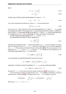
β 0 = µ Y − µ X ρ , (4.17)
σ X
σ Y
β 1 = , ρ (4.18)
σ X
and the variance of the conditional distribution of Y given X = x is

2
2
σ 2 = σ (1 − ρ ). (4.19)
Y |x Y
That is, the conditional distribution of Y given X = x is normal with mean

E(Y |x) = β 0 + β 1 x (4.20)

and variance σ 2 . Thus, the mean of the conditional distribution of Y given X = x is a simple
Y |x
linear regression model. Furthermore, there is a relationship between the correlation coefficient ρ
and the slope β 1 . From Equation (4.18) we see that if ρ = 0, then β 1 = 0, which implies that there
is no regression of Y on X. That is, knowledge of X does not assist us in predicting Y.
It is often useful to test the hypotheses H 0 : ρ = 0 and H 1 : ρ ̸= 0
The appropriate test statistic for these hypotheses is

√
R n − 2
T 0 = √ (4.21)
1 − R 2
which has the t distribution with n−2 degrees of freedom if H 0 : ρ = 0 is true. Therefore, we would
reject the null hypothesis if |t 0 | > t α/2,n−2 . This test is equivalent to the test of the hypothesis
H 0 : β 1 = 0. This equivalence follows directly from Equation (4.21). The test procedure for the
hypotheses H 0 : ρ = ρ 0 and H 1 : ρ ̸= ρ 0 where ρ 0 ̸= 0 is somewhat more complicated. For
moderately large samples (say, n ≥ 25), the statistic

1 1 + R
Z = artanh R = ln (4.22)
2 1 − R
is approximately normally distributed with mean and variance

1 1 + ρ 1
2
µ Z = artanh ρ = ln and σ =
Z
2 1 − ρ n − 3
respectively. Therefore, to test the hypothesis H 0 : ρ = ρ 0 , we may use the test statistic
√
Z 0 = (artanh R − artanh ρ 0 ) n − 3 (4.23)

and reject H 0 : ρ = ρ 0 if the value of the test statistic in Equation (4.23) is such that |z 0 | > z α/2 .
It is also possible to construct an approximate 100(1−α)% confidence interval for ρ, using the
transformation in Equation (4.22). The approximate 100(1 − α)% confidence interval is

( ) ( )
z α/2 z α/2
tanh artanh r − √ ≤ ρ ≤ tanh artanh r + √
n − 3 n − 3
u
u
where tanh u = (e − e −u )/(e + e −u ).

114