Page 112 - 4660

Simple linear regression and correlation

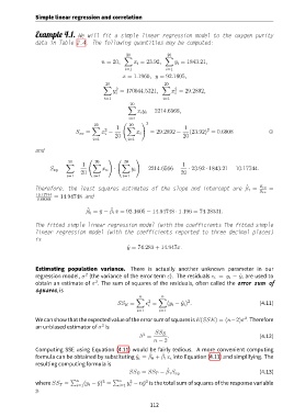
Example 4.1. We will fit a simple linear regression model to the oxygen purity
data in Table 2.4. The following quantities may be computed:

20 20
∑ ∑
n = 20, x i = 23.92, y i = 1843.21,
i=1 i=1
¯ x = 1.1960, ¯y = 92.1605,
20 20
∑ 2 ∑ 2
y = 170044.5321, x = 29.2892,
i
i
i=1 i=1
20
∑
x i y i = 2214.6566,
i=1
( ) 2
20 20
∑ 1 ∑ 1
2
2
S xx = x − x i = 29.2892 − (23.92) = 0.6808 ,
i
i=1 20 i=1 20
and
( ) ( )
20 20 20
∑ 1 ∑ ∑ 1
S xy = − x u · y i = 2214.6566 − · 23.92 · 1843.21 = 10.17744.
20 20
i=1 i=1 i=1
ˆ
Therefore, the least squares estimates of the slope and intercept are β 1 = S xy =
S xx
10.17744 = 14.94748 and
0.68088
ˆ
ˆ
β 0 = ¯y − β 1 ¯x = 92.1605 − 14.94748 · 1.196 = 74.28331.
The fitted simple linear regression model (with the coefficients The fitted simple
linear regression model (with the coefficients reported to three decimal places)
is
ˆ y = 74.283 + 14.947x.

Estimating population variance. There is actually another unknown parameter in our
2
regression model, σ (the variance of the error term ε). The residuals e i = y i − ˆy i are used to
obtain an estimate of σ . The sum of squares of the residuals, often called the error sum of
2
squares, is
n n
∑ ∑
2
2
SS E = e = (y i − ˆy i ) . (4.11)
i
i=1 i=1
2
Wecanshowthat theexpectedvalueof theerrorsumof squaresis E(SSE) = (n−2)σ . Therefore
2
an unbiased estimator of σ is
2
ˆ σ = SS E . (4.12)
n − 2
Computing SSE using Equation (4.11) would be fairly tedious. A more convenient computing
ˆ
ˆ
formula can be obtained by substituting ˆy i = β 0 + β 1 x i into Equation (4.11) and simplifying. The
resulting computing formula is
ˆ (4.13)
SS E = SS T − β 1 S xy
∑ n 2 ∑ n 2 2
where SS T = (y i − ¯y) = y − n¯y is the total sum of squares of the response variable
i=1 i=1 i
y.

112