Page 104 - 4660

Hypothesis testing

∫
where we have used the condition ∞ P(t|H 0 )dt = 1 to determine the normalisation constant.
−∞
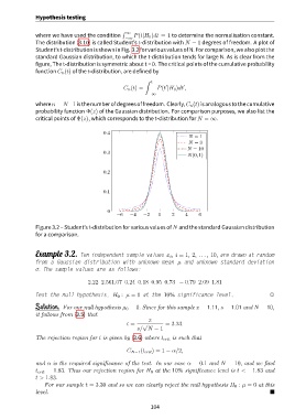
The distribution (3.10) is called Student’s t-distribution with N − 1 degrees of freedom. A plot of
Student’st-distributionisshowninFig. 3.2forvariousvaluesofN.Forcomparison, wealsoplotthe
standard Gaussian distribution, to which the t-distribution tends for large N. As is clear from the
figure, The t-distribution is symmetric about t = 0. The critical points of the cumulative probability
function C n (t) of the t-distribution, are defined by

∫ t
C n (t) = P(t |H 0 )dt ,
′
′
−∞
wheren = N−1isthenumberofdegreesoffreedom. Clearly,C n (t)isanalogoustothecumulative
probability function Φ(z) of the Gaussian distribution. For comparison purposes, we also list the
critical points of Φ(z), which corresponds to the t-distribution for N = ∞.

0.4
N = 1
N = 3
N = 10
0.3
N(0, 1)

0.2

0.1

0
−6 −4 −2 0 2 4 6
Figure 3.2 – Student’s t-distribution for various values of N and the standard Gaussian distribution
for a comparison.

Example 3.2. Ten independent sample values x i , i = 1, 2, . . . , 10, are drawn at random
from a Gaussian distribution with unknown mean µ and unknown standard deviation
σ. The sample values are as follows:

2.22 2.561.07 0.24 0.18 0.95 0.73 − 0.79 2.09 1.81

Test the null hypothesis, H 0 : µ = 0 at the 10% significance level. ,

Solution. For our null hypothesis µ 0 = 0. Since for this sample ¯x = 1.11, s = 1.01 and N = 10,
it follows from (3.5) that
¯ x
t = √ = 3.33.
s/ N − 1
The rejection region for t is given by (3.6) where t crit is such that

C N−1 (t crit ) = 1 − α/2,

and α is the required significance of the test. In our case α = 0.1 and N = 10, and we find
t crit = 1.83. Thus our rejection region for H 0 at the 10% significance level is t < −1.83 and
t > 1.83.
For our sample t = 3.30 and so we can clearly reject the null hypothesis H 0 : µ = 0 at this
level.

104