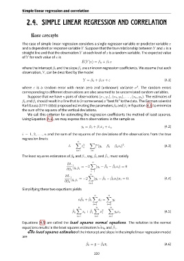
Page 110 - 4660

Simple linear regression and correlation

2.4. Simple linear regression and correlation

Base concepts

The case of simple linear regression considers a single regressor variable or predictor variable x
and a dependent or response variable Y. Suppose that the true relationship between Y and x is a
straight line and that the observation Y at each level of x is a random variable. The expected value
of Y for each value of x is
E(Y |x) = β 0 + β 1 x

where the intercept β 0 and the slope β 1 are unknown regression coefficients. We assume that each
observation, Y, can be described by the model

Y = β 0 + β 1 x + ε (4.1)

2
where ε is a random error with mean zero and (unknown) variance σ . The random errors
corresponding to different observations are also assumed to be uncorrelated random variables.
Suppose that we have n pairs of observations (x 1 , y 1 ), (x 2 , y 2 ), . . . , (x n , y n ). The estimates of
β 0 and β 1 should result in a line that is (in some sense) a ”best fit” to the data. The German scientist
KarlGauss(1777-1855)proposedestimatingtheparametersβ 0 andβ 1 inEquation(4.1)tominimize
the sum of the squares of the vertical deviations.
We call this criterion for estimating the regression coefficients the method of least squares.
Using Equation (4.1), we may express the n observations in the sample as

y i = β 0 + β 1 x j + ε i , (4.2)

i = 1, 2, . . . , n and the sum of the squares of the deviations of the observations from the true
regression line is
n
∑ ∑
2
2
n
L = ε = ] (y i − β 0 − β 1 x i ) . (4.3)
i
i=1 i=
ˆ
ˆ
The least squares estimators of β 0 and β 1 , say, β 0 and β 1 , must satisfy
n
∂L ∑
ˆ
ˆ
= −2 (y i − β 0 − β 1 x i ) = 0
ˆ ˆ
β 0 ,β 1
∂β 0
i=1
n
∂L ∑
ˆ
ˆ
= −2 (y i − β 0 − β 1 x i )x i = 0. (4.4)
ˆ ˆ
β 0 ,β 1
∂β 1
i=1
Simplifying these two equations yields
n n
∑ ∑
ˆ ˆ
nβ 0 + β 1 x i = y i
i=1 i=1
n n n
∑ ∑ ∑
ˆ ˆ 2
β 0 x i + β 1 x = y i x i . (4.5)
i
i=1 i=1 i=1
Equations (4.5) are called the least squares normal equations. The solution to the normal
ˆ
ˆ
equations results in the least squares estimators beta 0 and β 1 .
The least squares estimates of the intercept and slope in the simple linear regression model
are
ˆ
ˆ
β 0 = ¯y − β 1 ¯x, (4.6)
110