Page 42 - 6653

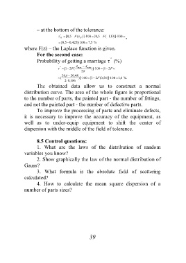
– at the bottom of the tolerance:
 ' H  5 , 0 [  F (z H )] 100  5 , 0 [  F ( , 1 13 )] 100  ,
 5 , 0 [  , 0 425 ] 100  5 , 7 %
where F(z) – the Laplace function is given.
For the second case:
’’
Probability of getting a marriage  (%)
A max  A
 ' '  1 [  2F ( min )] 100 1 [  2 F
2
20 6 ,  20 , 48
(  )] 100 1 [  2F , 0 ( 56 )] 100  4 , 1 %.
2 , 0  106
The obtained data allow us to construct a normal
distribution curve. The area of the whole figure is proportional
to the number of parts, the painted part - the number of fittings,
and not the painted part - the number of defective parts.
To improve the processing of parts and eliminate defects,
it is necessary to improve the accuracy of the equipment, as
well as to under-equip equipment to shift the center of
dispersion with the middle of the field of tolerance.

8.5 Control questions:
1. What are the laws of the distribution of random
variables you know?
2. Show graphically the law of the normal distribution of
Gauss?
3. What formula is the absolute field of scattering
calculated?
4. How to calculate the mean square dispersion of a
number of parts sizes?

39