Page 28 - 6099

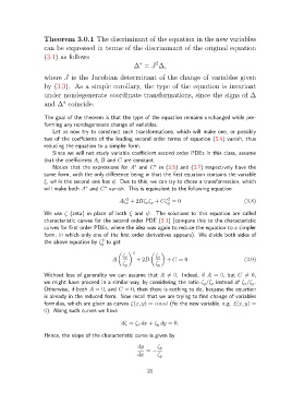
Theorem 3.0.1 The discriminant of the equation in the new variables

can be expressed in terms of the discriminant of the original equation
(3.1) as follows
2
∗
∆ = J ∆,
where J is the Jacobian determinant of the change of variables given
by (3.3). As a simple corollary, the type of the equation is invariant

under nondegenerate coordinate transformations, since the signs of ∆
and ∆ coincide.
∗
The goal of the theorem is that the type of the equation remains unchanged while per-
forming any nondegenerate change of variables.
Let us now try to construct such transformations, which will make one, or possibly
two of the coeffcients of the leading second order terms of equation (3.4) vanish, thus
reducing the equation to a simpler form.
Since we will not study variable coefficient second order PDEs in this class, assume
that the coefficients A, B and C are constant.
∗
∗
Notice that the expressions for A and C in (3.5) and (3.7) respectively have the
same form, with the only difference being in that the first equation contains the variable
ξ, while the second one has ψ. Due to this, we can try to chose a transformation, which
∗
∗
will make both A and C vanish. This is equivalent to the following equation
2
2
Aζ + 2Bζ x ζ y + Cζ = 0 (3.8)
x y
We use ζ (zeta) in place of both ξ and ψ. The solutions to this equation are called
characteristic curves for the second order PDE (3.1) (compare this to the characteristic
curves for first order PDEs, where the idea was again to reduce the equation to a simpler
form, in which only one of the first order derivatives appears). We divide both sides of
2
the above equation by ζ to get
y
2

ζ x ζ x
A + 2B + C = 0 (3.9)
ζ y ζ y
Without loss of generality we can assume that A 6= 0. Indeed, if A = 0, but C 6= 0,
we might have proceed in a similar way, by considering the ratio ζ y /ζ x instead of ζ x /ζ y .
Otherwise, if both A = 0, and C = 0, then there is nothing to do, because the equation
is already in the reduced form. Now recall that we are trying to find change of variables
formulas, which are given as curves ζ(x, y) = const (fix the new variable, e.g. ξ(x, y) =
0). Along such curves we have

dζ = ζ x dx + ζ y dy = 0.

Hence, the slope of the characteristic curve is given by

dy ζ x
= −
dx ζ y

21