Page 35 - 4660

1.5. Discrete random variables

Suppose an experiment has an outcome sample space S. A real variable X that is defined for
all possible outcomes in S (so that a real number — not necessarily unique — is assigned to each
possible outcome) is called a random variable (RV). The outcome of the experiment may
already be a real number and hence a random variable, e.g. the number of heads obtained in 10
throws of a coin, or the sum of the values if two dice are thrown. However, more arbitrary
assignments are possible, e.g. the assignment of a ’quality’ rating to each successive item
produced by a manufacturing process. Furthermore, assuming that a probability can be assigned
to all possible outcomes in a sample space S, it is possible to assign a probability distribution

to any random variable. Random variables may be divided into two classes, discrete and
continuous, and we now examine each of these in turn.

General Definitions

Definition 5.1. A random variable is a variable, which assumes as a result of a
trial depending on casual circumstances. ✓

Definition 5.2. A random variable is said to be discrete if it takes only a finite
or countable infinite number of values x i with probabilities p i .

Definition 5.3. A random variable is said to be continuous if it takes all values in
some finite or infinite interval, that is values completely fill some interval (finite
or infinite).

An example of a discrete random variable is the number of heads obtained in 10 throws of a
coin.
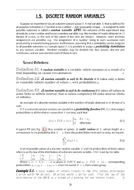
If X is a discrete random variable, we can define aprobability function (PF) f(x) that assigns
probabilities to all the distinct values that X can take, such that
{
if x = x i ,
p i
f(x) = P(X = x) = (5.1)
0 otherwise .

A typical PF (see Fig. 5.1) thus consists of spikes, at valid values of X, whose height at x
corresponds to the probability that X = x. Since the probabilities must sum to unity, we require

n
∑
f(x i ) = 1. (5.2)
i=1

A set of possible values of a discrete random variable X and the probabilities of these values
refers to as the law of the distribution of a discrete random variable. DRV is set by the table
X x 1 x 2 … x n
P p 1 p 2 … p n
Where x i (i = 1, 2, . . . , n) a values of DRV X and p i = P(X = x i ) — corresponding
probabilities. p 1 + p 2 + . . . + p n = 1, since the events X = x i form a total group.

Example 5.1. A total number of lottery tickets is 100. This lottery distributes
1 prize worth 50 dollars, 10 prizes worth 1 dollar each. Find the law of the
distribution of the RV X as a volume of a winning for one lottery ticket. ,

35