Page 100 - 4660

Hypothesis testing

P(t|H 0 )

α

t
0 t crit
P(t|H 1 )

β

t
0 t crit
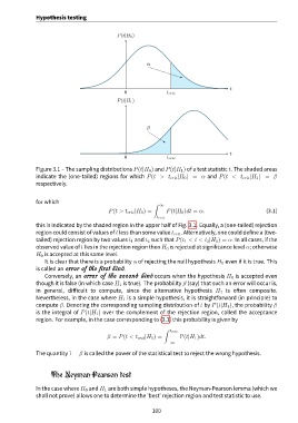
Figure 3.1 – The sampling distributions P(t|H 0 ) and P(t|H 1 ) of a test statistic t. The shaded areas
indicate the (one-tailed) regions for which P(t > t crit |H 0 ) = α and P(t < t crit |H 1 ) = β
respectively.

for which
∫
∞
P(t > t crit |H 0 ) = P(t|H 0 )dt = α. (3.1)
t crit
this is indicated by the shaded region in the upper half of Fig. 3.1. Equally, a (one-tailed) rejection
region could consist of values of t less than some value t crit . Alternatively, one could define a (two-
tailed) rejection region by two values t 1 and t 2 such that P(t 1 < t < t 2 |H 0 ) = α. In all cases, if the
observed value of t lies in the rejection region then H 0 is rejected at significance level α; otherwise
H 0 is accepted at this same level.
It is clear that there is a probability α of rejecting the null hypothesis H 0 even if it is true. This
is called an error of the first kind.
Conversely, an error of the second kind occurs when the hypothesis H 0 is accepted even
though it is false (in which case H 1 is true). The probability β (say) that such an error will occur is,
in general, difficult to compute, since the alternative hypothesis H 1 is often composite.
Nevertheless, in the case where H 1 is a simple hypothesis, it is straightforward (in principle) to
compute β. Denoting the corresponding sampling distribution of t by P(t|H 1 ), the probability β
is the integral of P(t|H 1 ) over the complement of the rejection region, called the acceptance
region. For example, in the case corresponding to (3.1) this probability is given by

∫
t crit
β = P(t < t crit |H 1 ) = P(t|H 1 )dt.
−∞
The quantity 1 − β is called the power of the statistical test to reject the wrong hypothesis.

The Neyman-Pearson test

In the case where H 0 and H 1 are both simple hypotheses, the Neyman-Pearson lemma (which we
shall not prove) allows one to determine the ’best’ rejection region and test statistic to use.

100