Page 82 - 6685

 B 

Q  ln r   ln n inj  

w
inj
n   2 rw inj   . (4.10)
inj
2 k  w h Р bh inj  Р line
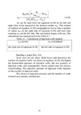
As can be seen from the equation (4.10) in the left and
right sides of the equation is the desired number n inj. The method
of solution of equation (4.10) semigraphical. Let us take a number
of values n inj on the right side of equation (4.10) and each time
counting n inj on the left side. The calculation begins with one. The
calculations are summarized in the Table 4.1.
Table 4.1 – Calculation of injection wells number
n inj (given) n inj (calculated)

the right side of equation (4.10) the left side of equation (4.10)

Building a graph (Fig. 4.8).
Scale axes are the same. Hold bisect and determine the
number of injection wells. As shown in equation (4.10), the higher
the bottom-hole pressure of injection wells, the less quantity of
injection wells, and consequently, lower capital costs for process
waterflooding. The injection pressure of injection wells depends
on the number of injection wells.
The choice of injection pressure and the number of wells
is based on economic calculations.

82